MLIR 파트 4 - MLIR의 선형대수

Linalg 방언은 MLIR 생태계의 핵심 아이디어로, 고수준 텐서 계산을 더 쉽고 더 효율적으로 만들기 위해 구축되었다. 본질적으로 이는 복잡한 수학 연산을 다루는 방식을 단순화하여 빠르고 최적화된 코드로 변환될 수 있게 하는 데 초점이 있다. Linalg 방언은 핵심에서 간단하고 선언적인 접근 방식을 사용한다. 즉, 수학적 의미를 유지하면서도 다양한 최적화를 허용하는 형태로 연산과 변환을 서술한다. 점별(pointwise) 계산, 행렬 곱, 컨볼루션 같은 고수준 선형대수 연산을 단일 연산으로 제공한다.

linalg.generic

Linalg 방언에서 가장 범용적인 연산은 linalg.generic이다. 이 연산은 인덱스에 대해 일반적인 텐서 조작 연산을 정의할 수 있게 해준다. 이것이 가장 일반적인 연산이며, 다른 모든 연산은 이 연산의 특수화로 정의된다. 아마 이를 직접 많이 쓰지는 않겠지만, 가장 근본적인 연산이므로 먼저 논의하는 것이 유용하다.

#map_1d_identity = affine_map<(d0) -> (d0)>

func.func @add_tensors(%arg0: tensor<10xf32>, %arg1: tensor<10xf32>) -> tensor<10xf32> {
  %result = tensor.empty() : tensor<10xf32>
  %0 = linalg.generic {
    // attributes
      indexing_maps = [
        #map_1d_identity,
        #map_1d_identity,
        #map_1d_identity
       ],
      iterator_types = [
        "parallel"
      ]
    } 
    // input tensors
    ins(%arg0, %arg1 : tensor<10xf32>, tensor<10xf32>) 
    // output tensor
    outs(%result : tensor<10xf32>) 
    // loop region
    {
    ^bb0(%arg2: f32, %arg3: f32, %arg4: f32):
      %1 = arith.addf %arg2, %arg3 : f32
      linalg.yield %1 : f32
    } -> tensor<10xf32>
  return %0 : tensor<10xf32>
}

이 linalg.generic 연산의 각 구성 요소를 나눠 보자.

1. indexing_maps: 이 속성은 입력 및 출력 텐서에 어떻게 접근하는지를 정의한다. 여기에는 3개의 맵이 있다.

   • 첫 번째 입력 텐서(%arg0)를 위한 첫 번째 맵
   • 두 번째 입력 텐서(%arg1)를 위한 두 번째 맵
   • 출력 텐서(%result)를 위한 세 번째 맵

모두 #map_1d_identity를 사용하는데, 이는 affine_map<(d0) -> (d0)>로 정의되어 있으며 각 원소가 대응하는 원소로 직접 매핑됨(좌표 변환 없음)을 의미한다.

2. iterator_types: 각 차원에 대한 반복(iteration) 타입을 지정한다. 여기서는 다음이 있다.

   • ["parallel"]: 단일 차원을 병렬로 표시하며, 반복들이 어떤 순서로든 또는 동시에 실행될 수 있음을 뜻한다.

linalg에는 가능한 iterator 타입이 세 가지 있다.

*   `parallel`: 반복을 어떤 순서로든 또는 동시에 실행할 수 있음(원소별 연산 같은 경우)
*   `reduction`: 반복이 단일 결과 값에 기여함(어떤 축을 따라 합산하는 경우)
*   `window`: 반복이 원소의 슬라이딩 윈도우에 접근함(컨볼루션 같은 경우)

3. ins(%arg0, %arg1 : tensor<10xf32>, tensor<10xf32>):

*   입력 텐서들과 그 타입을 지정한다.
*   둘 다 10개의 float32 원소로 이루어진 1D 텐서이다.

4. outs(%result : tensor<10xf32>):

*   출력 텐서와 그 타입을 지정한다.
*   이 또한 10개의 float32 원소로 이루어진 1D 텐서이다.

5. 리전(루프 본문):

{
^bb0(%arg2: f32, %arg3: f32, %arg4: f32):
  %1 = arith.addf %arg2, %arg3 : f32
  linalg.yield %1 : f32
}

*   입력 텐서(%arg2, %arg3)와 출력 텐서(%arg4)에서 스칼라 값을 받는다.
*   부동소수점 덧셈을 수행한다.
*   `linalg.yield`를 사용해 결과를 다시 반환한다.

이는 NumPy에서처럼 두 텐서를 원소별로 더하는 표준 벡터화 덧셈을 수행한다.

np.array([1,2,3]) + np.array([2,3,4])
# array([3, 5, 7])

이게 너무 많아 보인다면 걱정하지 않아도 된다. 실제로 많다. 동일한 것으로 컴파일되는 훨씬 더 간단한 작성 방법들이 있다.

linalg.map

같은 연산을 범용 linalg.map 연산으로 작성할 수도 있는데, 이는 루프 중첩과 인덱스 조작의 정확한 세부사항을 추상화하고 대신 입력 텐서에 arith.addf 연산을 직접 적용한다.

module {
  func.func @addv(%arg0: tensor<10xf32>, %arg1: tensor<10xf32>, %out: memref<10xf32>) {
    %out2 = tensor.empty() : tensor<10xf32>
    %result = linalg.map { arith.addf } ins(%arg0, %arg1 : tensor<10xf32>, tensor<10xf32>) outs(%out2 : tensor<10xf32>)

    %l = bufferization.to_memref %result : tensor<10xf32> to memref<10xf32>
    memref.copy %l, %out : memref<10xf32> to memref<10xf32>

    return
  }
}

또한 일반적인 산술 맵 연산을 위한 이름 있는 연산들도 있는데, 이는 linalg.map 연산의 이름 있는 특수화이다.

• linalg.add
• linalg.mul
• linalg.div
• linalg.sub

linalg.reduce

linalg.reduce 연산은 다양한 리덕션 연산을 구현하는 데 사용할 수 있는 강력한 프리미티브이다.

func.func @add_tensor() -> (f64) {
  %_ssa_0 = tensor.empty () : tensor<3xf64>
  %out = tensor.empty () : tensor<f64>
  %reduce = linalg.reduce { arith.addf } ins(%_ssa_0:tensor<3xf64>) outs(%out:tensor<f64>) dimensions = [0]
  %result = tensor.extract %reduce [] : tensor<f64>
  return %result : f64
}

NumPy에서는 이 연산을 다음처럼 쓸 수 있다.

import numpy as np
np.multiply.reduce([2,3,5]) # 30

linalg.matmul

직접적인 텐서 컨트랙션으로 일반적인 행렬 곱 연산을 정의할 수도 있다. MLIR 코드에 나타난 행렬 곱 연산은 전통적인 텐서 표기법으로 다음과 같이 쓸 수 있다.

C i j=∑k=1 10 A i k B k j

여기서:

• A는 8×10 입력 행렬이다(memref<8x10xf32>).
• B는 10×16 입력 행렬이다(memref<10x16xf32>).
• C는 8×16 출력 행렬이다(memref<8x16xf32>).
• i는 1부터 8까지 범위를 갖는다.
• j는 1부터 16까지 범위를 갖는다.
• k는 1부터 10까지 범위를 갖는 합산 인덱스이다.

이는 MLIR 구현과 일치하는데, 그 이유는 다음과 같다.

• parallel iterator 타입은 자유 인덱스 i와 j에 대응한다.
• reduction iterator 타입은 k에 대한 합산에 대응한다.
• 인덱싱 맵 (i, j, k) -> (i, k), (i, j, k) -> (k, j), (i, j, k) -> (i, j)는 각각 A i k, B k j, C i j에 접근하는 것에 대응한다.

func.func @matmul(
    %A: memref<8x10xf32>,
    %B: memref<10x16xf32>,
    %C: memref<8x16xf32>
) {
    linalg.generic {
        indexing_maps = [
            affine_map<(i, j, k) -> (i, k)>,
            affine_map<(i, j, k) -> (k, j)>,
            affine_map<(i, j, k) -> (i, j)>
        ],
        iterator_types = [
            "parallel",
            "parallel",
            "reduction"
        ]
    } ins(%A, %B : memref<8x10xf32>, memref<10x16xf32>) outs(%C : memref<8x16xf32>) {
        ^bb0(%lhs_one: f32, %rhs_one: f32, %init_one: f32):
            %tmp0 = arith.mulf %lhs_one, %rhs_one : f32
            %tmp1 = arith.addf %init_one, %tmp0 : f32
            linalg.yield %tmp1 : f32
    }
    return
}

또는 linalg.matmul 연산을 사용하는 훨씬 더 간결한 형태로도 쓸 수 있다.

func.func @matmul(
    %A: memref<8x10xf32>,
    %B: memref<10x16xf32>,
    %C: memref<8x16xf32>
) {
    linalg.matmul ins(%A, %B : memref<8x10xf32>, memref<10x16xf32>) outs(%C : memref<8x16xf32>)
    return
}

그 다음 텐서 연산은 convert-linalg-to-loops 또는 convert-linalg-to-affine-loops 패스를 사용하여 affine.for 또는 scf.for 연산으로 이루어진 루프 시퀀스로 로워링된다.

func.func @matmul(%arg0: memref<8x10xf32>, %arg1: memref<10x16xf32>, %arg2: memref<8x16xf32>) {
  affine.for %arg3 = 0 to 8 {
    affine.for %arg4 = 0 to 16 {
      affine.for %arg5 = 0 to 10 {
        %0 = affine.load %arg0[%arg3, %arg5] : memref<8x10xf32>
        %1 = affine.load %arg1[%arg5, %arg4] : memref<10x16xf32>
        %2 = affine.load %arg2[%arg3, %arg4] : memref<8x16xf32>
        %3 = arith.mulf %0, %1 : f32
        %4 = arith.addf %2, %3 : f32
        affine.store %4, %arg2[%arg3, %arg4] : memref<8x16xf32>
      }
    }
  }
  return
}

func.func @matmul(%arg0: memref<8x10xf32>, %arg1: memref<10x16xf32>, %arg2: memref<8x16xf32>) {
  %c0 = arith.constant 0 : index
  %c8 = arith.constant 8 : index
  %c1 = arith.constant 1 : index
  %c16 = arith.constant 16 : index
  %c10 = arith.constant 10 : index
  scf.for %arg3 = %c0 to %c8 step %c1 {
    scf.for %arg4 = %c0 to %c16 step %c1 {
      scf.for %arg5 = %c0 to %c10 step %c1 {
        %0 = memref.load %arg0[%arg3, %arg5] : memref<8x10xf32>
        %1 = memref.load %arg1[%arg5, %arg4] : memref<10x16xf32>
        %2 = memref.load %arg2[%arg3, %arg4] : memref<8x16xf32>
        %3 = arith.mulf %0, %1 : f32
        %4 = arith.addf %2, %3 : f32
        memref.store %4, %arg2[%arg3, %arg4] : memref<8x16xf32>
      }
    }
  }
  return
}

Broadcasting

MLIR의 Linalg 방언에서 브로드캐스팅은 NumPy의 브로드캐스팅 규칙과 유사하게, 서로 다른 shape의 텐서를 결합해 연산할 수 있게 해준다. 작은 텐서는 브로드캐스트 차원을 따라 더 큰 텐서의 shape에 맞도록 암묵적으로 확장된다. 이는 행렬의 각 행/열에 벡터를 더하거나 텐서에 스칼라 연산을 적용하는 같은 연산에 특히 유용하다.

몇 가지 흔한 브로드캐스팅 패턴을 살펴보자.

func.func @broadcast_1d_to_2d(%arg0: tensor<3xf32>) -> tensor<3x3xf32> {
  // Create an empty output tensor
  %init = tensor.empty() : tensor<3x3xf32>
  
  // Broadcast the input tensor along dimension 1 (columns)
  %result = linalg.broadcast 
    ins(%arg0: tensor<3xf32>)
    outs(%init: tensor<3x3xf32>)
    dimensions = [1]
    
  return %result : tensor<3x3xf32>
}

NumPy에서는 이 연산을 다음처럼 쓸 수 있다.

arg0 = np.array([1,2,3])
result = np.broadcast_to(arg0, (3,3))
# array([[1, 2, 3],
#        [1, 2, 3],
#        [1, 2, 3]])

브로드캐스팅을 다른 연산과 결합할 수도 있다. 예를 들어 행렬의 각 행에 벡터를 더하는 경우이다.

func.func @add_vector_to_matrix(
    %matrix: tensor<3x4xf32>,
    %vector: tensor<4xf32>
) -> tensor<3x4xf32> {
  %init = tensor.empty() : tensor<3x4xf32>
  
  // First broadcast the vector
  %broadcasted = linalg.broadcast
    ins(%vector: tensor<4xf32>)
    outs(%init: tensor<3x4xf32>)
    dimensions = [0]
    
  // Then add the broadcasted result to the matrix
  %result = linalg.map { arith.addf }
    ins(%matrix, %broadcasted: tensor<3x4xf32>, tensor<3x4xf32>)
    outs(%init: tensor<3x4xf32>)
    
  return %result : tensor<3x4xf32>
}

이는 흔히 쓰는 NumPy 연산과 동등하다.

matrix = np.ones((3,4))
vector = np.array([1,2,3,4])
result = matrix + vector
# array([[2., 3., 4., 5.],
#        [2., 3., 4., 5.],
#        [2., 3., 4., 5.]])

Kernel Fusion

커널 퓨전은 여러 연산을 하나의 연산으로 결합하여 메모리 대역폭 요구를 줄이고 성능을 향상시키는 중요한 최적화 기법이다. Linalg 방언은 최적화 패스를 통해 원소별 연산을 퓨전하는 기능을 내장 지원한다.

덧셈 다음에 곱셈을 수행하는 두 연산을 함께 퓨전하고 싶은 간단한 예를 보자. 먼저 이를 개별 연산으로 작성해 보자.

module {
  func.func @addmul(%arg0: tensor<10xf32>, %arg1: tensor<10xf32>, %arg2: tensor<10xf32>) -> tensor<10xf32> {
    // First create an empty tensor for intermediate results
    %0 = tensor.empty() : tensor<10xf32>
    
    // Add operation
    %1 = linalg.add ins(%arg0, %arg1 : tensor<10xf32>, tensor<10xf32>)
                    outs(%0 : tensor<10xf32>) -> tensor<10xf32>

    // Create another empty tensor for the multiplication result
    %2 = tensor.empty() : tensor<10xf32>
    
    // Multiply operation
    %3 = linalg.mul ins(%1, %arg2 : tensor<10xf32>, tensor<10xf32>)
                    outs(%2 : tensor<10xf32>) -> tensor<10xf32>

    return %3 : tensor<10xf32>
  }
}

여기에는 linalg.add 다음에 linalg.mul이라는 두 개의 서로 구분된 연산이 있다. 각 연산은 메모리에서 읽고 다시 메모리에 쓰는 것을 요구하며, 이는 비효율적일 수 있다.

MLIR의 최적화 패스를 통해, 이 연산들은 데이터 위를 한 번만 순회하면서 두 연산을 모두 수행하는 단일 커널로 퓨전할 수 있다.

#map = affine_map<(d0) -> (d0)>
module {
  func.func @addmul(%arg0: tensor<10xf32>, %arg1: tensor<10xf32>, %arg2: tensor<10xf32>) -> tensor<10xf32> {
    %0 = tensor.empty() : tensor<10xf32>
    %1 = linalg.generic {indexing_maps = [#map, #map, #map, #map],
        iterator_types = ["parallel"]} ins(%arg0, %arg1, %arg2 : tensor<10xf32>,
        tensor<10xf32>, tensor<10xf32>) outs(%0 : tensor<10xf32>) {
    ^bb0(%in: f32, %in_0: f32, %in_1: f32, %out: f32):
      %2 = arith.addf %in, %in_0 : f32
      %3 = arith.mulf %2, %in_1 : f32
      linalg.yield %3 : f32
    } -> tensor<10xf32>
    return %1 : tensor<10xf32>
  }
}

이게 어떻게 동작하는지 직관을 얻기 위해, 동등한 Python 코드를 보자.

# Unfused version - two separate loops
def unfused_addmul(a, b, c):
    # First loop - addition
    temp = []
    for i in range(len(a)):
        temp.append(a[i] + b[i])
    
    # Second loop - multiplication
    result = []
    for i in range(len(temp)):
        result.append(temp[i] * c[i])
    
    return result

# Fused version - single loop
def fused_addmul(a, b, c):
    result = []
    for i in range(len(a)):
        # Combine add and multiply in one loop iteration
        result.append((a[i] + b[i]) * c[i])
    return result

a = [1.0, 2.0, 3.0, 4.0, 5.0]
b = [1.0, 1.0, 1.0, 1.0, 1.0]
c = [2.0, 2.0, 2.0, 2.0, 2.0]

# Both produce same result but fused version only loops once
result = fused_addmul(a, b, c)  # [(1+1)*2, (2+1)*2, (3+1)*2, ...]

퓨전된 버전은 두 연산을 단일 linalg.generic 연산으로 결합하여 각 입력을 한 번만 읽고 최종 결과를 직접 기록한다. 이렇게 하면 중간 텐서 할당과 메모리 접근이 제거된다.

이 퓨전을 수행하려면 특정한 최적화 패스 시퀀스를 적용해야 한다.

1. --canonicalize: 일반적인 정리 및 단순화를 수행
2. --linalg-fuse-elementwise-ops: 원소별 연산을 퓨전
3. --cse: 중복 연산을 정리하기 위한 공통 부분식 제거(Common Subexpression Elimination)
4. --linalg-generalize-named-ops: 이름 있는 연산(예: linalg.add)을 generic 형태로 변환
5. --convert-linalg-to-loops: 퓨전된 연산을 명시적 루프로 변환

이 패스들을 실행하고 퓨전된 addmul 연산을 fused_ops.mlir로 출력하여, n에 대해 두 번 루프를 도는 시간 복잡도를 n에 대해 한 번만 도는 것으로 줄일 수 있다.

mlir-opt separate_ops.mlir \
  --canonicalize \
  --linalg-fuse-elementwise-ops \
  --cse \
  --linalg-generalize-named-ops \
  --linalg-fuse-elementwise-ops \
  --convert-linalg-to-loops \
  -o fused_ops.mlir

이 패스 시퀀스는 연산들이 올바르게 퓨전된 뒤 효율적으로 실행 가능한 형태로 로워링되도록 보장한다. 퓨전 최적화는 원소별 연산 체인이 흔한 딥러닝 워크로드에서 특히 중요하다.

Tiling

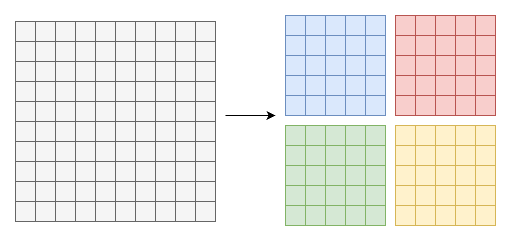
루프 타일링은 메모리 접근 패턴과 캐시 활용을 개선하는 데 핵심적인 최적화 기법이다. 현대 컴퓨터 아키텍처에서는 연산보다 메모리 접근이 병목인 경우가 흔하다. 큰 행렬이나 텐서를 처리할 때 메모리를 선형으로 접근하면 계속해서 메인 메모리에서 새 데이터를 가져와야 할 수 있는데, 이는 캐시 메모리보다 훨씬 느리다.

타일링은 큰 계산을 캐시에 더 잘 들어맞는 작은 블록으로 쪼갠다. 예를 들어 행렬 곱에서는 전체 행-열 내적을 한 번에 계산하는 대신(캐시 크기를 초과할 수 있음), 캐시에 상주할 수 있는 더 작은 타일로 나눈다. 이는 캐시 미스를 줄이고 성능을 개선한다.

이 최적화는 GPU 아키텍처에서 특히 중요한데, 메모리 계층과 접근 패턴이 성능에 큰 영향을 주기 때문이다. GPU에는 글로벌 메모리, 공유 메모리(캐시와 유사), 레지스터를 포함한 복잡한 메모리 계층이 있다. 연산을 GPU의 하드웨어 특성—예를 들어 공유 메모리 크기와 워프 크기—에 맞게 타일링하면 성능을 극적으로 개선할 수 있다. 예컨대 CUDA 프로그래밍에서는 데이터를 공유 메모리에 타일 단위로 로드하고, 스레드를 동기화한 뒤, 각 스레드가 해당 타일 내 원소를 처리하는 패턴이 흔하다. 이에 대해서는 뒤의 GPU 프로그래밍 섹션에서 더 다룬다.

다음은 MLIR을 사용해 행렬 곱 연산에 루프 타일링을 수행하는 예이다. 간단한 텐서 기반 matmul로 시작해, 이를 타일링된 affine 루프로 변환한다.

module {
  func.func @matmul(%arg0: tensor<10x10xf32>, %arg1: tensor<10x10xf32>,
                    %arg2: tensor<10x10xf32>) -> tensor<10x10xf32> {
    %0 = linalg.matmul 
           ins(%arg0, %arg1 : tensor<10x10xf32>, tensor<10x10xf32>)
           outs(%arg2 : tensor<10x10xf32>) -> tensor<10x10xf32>
    return %0 : tensor<10x10xf32>
  }
}

이를 타일링된 루프로 변환하려면 여러 변환 패스가 필요하다.

1. --convert-tensor-to-linalg: 텐서 연산을 linalg 방언으로 변환
2. --linalg-generalize-named-ops: 이름 있는 연산(예: matmul)을 generic linalg 연산으로 변환
3. --one-shot-bufferize="bufferize-function-boundaries": 텐서 연산이 버퍼를 사용하도록 변환
4. --buffer-deallocation-pipeline: 버퍼 해제를 처리
5. --convert-bufferization-to-memref: 버퍼 연산을 memref 연산으로 변환
6. --convert-linalg-to-affine-loops: linalg 연산을 affine 루프로 로워링
7. --affine-loop-tile="tile-size=5": 타일 크기 5로 affine 루프를 타일링
8. --canonicalize --cse: 정리 패스

전체 변환 파이프라인은 다음과 같다.

mlir-opt tiling.mlir \
  --convert-tensor-to-linalg \
  --linalg-generalize-named-ops \
  --one-shot-bufferize="bufferize-function-boundaries" \
  --buffer-deallocation-pipeline \
  --convert-bufferization-to-memref \
  --convert-linalg-to-affine-loops \
  --affine-loop-tile="tile-size=5" \
  --canonicalize \
  --cse \
  -o tiling-transformed.mlir

이는 다음과 같은 타일링된 구현을 생성한다.

#map = affine_map<(d0) -> (d0)>
#map1 = affine_map<(d0) -> (d0 + 5)>
module {
  func.func @matmul(%arg0: memref<10x10xf32, strided<[?, ?], offset: ?>>, %arg1:
  memref<10x10xf32, strided<[?, ?], offset: ?>>, %arg2: memref<10x10xf32,
  strided<[?, ?], offset: ?>>) -> memref<10x10xf32, strided<[?, ?], offset: ?>>
  {
    affine.for %arg3 = 0 to 10 step 5 {
      affine.for %arg4 = 0 to 10 step 5 {
        affine.for %arg5 = 0 to 10 step 5 {
          affine.for %arg6 = #map(%arg3) to #map1(%arg3) {
            affine.for %arg7 = #map(%arg4) to #map1(%arg4) {
              affine.for %arg8 = #map(%arg5) to #map1(%arg5) {
                %0 = affine.load %arg0[%arg6, %arg8] : memref<10x10xf32, strided<[?, ?], offset: ?>>
                %1 = affine.load %arg1[%arg8, %arg7] : memref<10x10xf32, strided<[?, ?], offset: ?>>
                %2 = affine.load %arg2[%arg6, %arg7] : memref<10x10xf32, strided<[?, ?], offset: ?>>
                %3 = arith.mulf %0, %1 : f32
                %4 = arith.addf %2, %3 : f32
                affine.store %4, %arg2[%arg6, %arg7] : memref<10x10xf32, strided<[?, ?], offset: ?>>
              }
            }
          }
        }
      }
    }
    %alloc = memref.alloc() : memref<10x10xf32>
    %cast = memref.cast %alloc : memref<10x10xf32> to memref<10x10xf32, strided<[?, ?], offset: ?>>
    memref.copy %arg2, %alloc : memref<10x10xf32, strided<[?, ?], offset: ?>> to memref<10x10xf32>
    return %cast : memref<10x10xf32, strided<[?, ?], offset: ?>>
  }
}

타일링된 출력은 원래 10x10 행렬 곱을 더 작은 5x5 타일로 쪼갠 것을 보여주며, 이는 캐시 활용과 메모리 접근의 지역성(locality)을 개선하는 데 도움이 될 수 있다.

External References

• MLIR: Linalg Dialect
• MLIR Open Meeting 2022-01-27: Introduction to Linalg.generic
• 2024 EuroLLVM - MLIR Linalg Op Fusion - Theory & Practice
• NumPy Broadcasting
• MLIR Codegen Dialects for Machine Learning Compilers
• MLIR Linalg Dialect and Patterns
• Linalg Dialect Rationale: The Case For Compiler-Friendly Custom Operations
• Anatomy of Linalg.generic
• IREE/MLIR/Linalg tutorial